Research | Lucia Pezzetti

Multi-Agent Reinforcement Learning

A Separation Principle for Cooperative Multi-Agent Reinforcement Learning

We study cooperative multi-agent reinforcement learning with decoupled noisy dynamics and a shared population objective. The separation principle upper-bounds the population cost-to-go by an optimal transport problem built from a target-conditioned single-agent cost-to-go. This leads to SALT: learn one reusable single-agent policy and coordinate the agents through optimal transport, enabling transfer across fleet sizes and stochastic mobility tasks.

Multi-agent RLOptimal transportFleet coordination

Illustration of data-driven control, transportation routes, and multi-agent system dynamics

The idea in one sentence

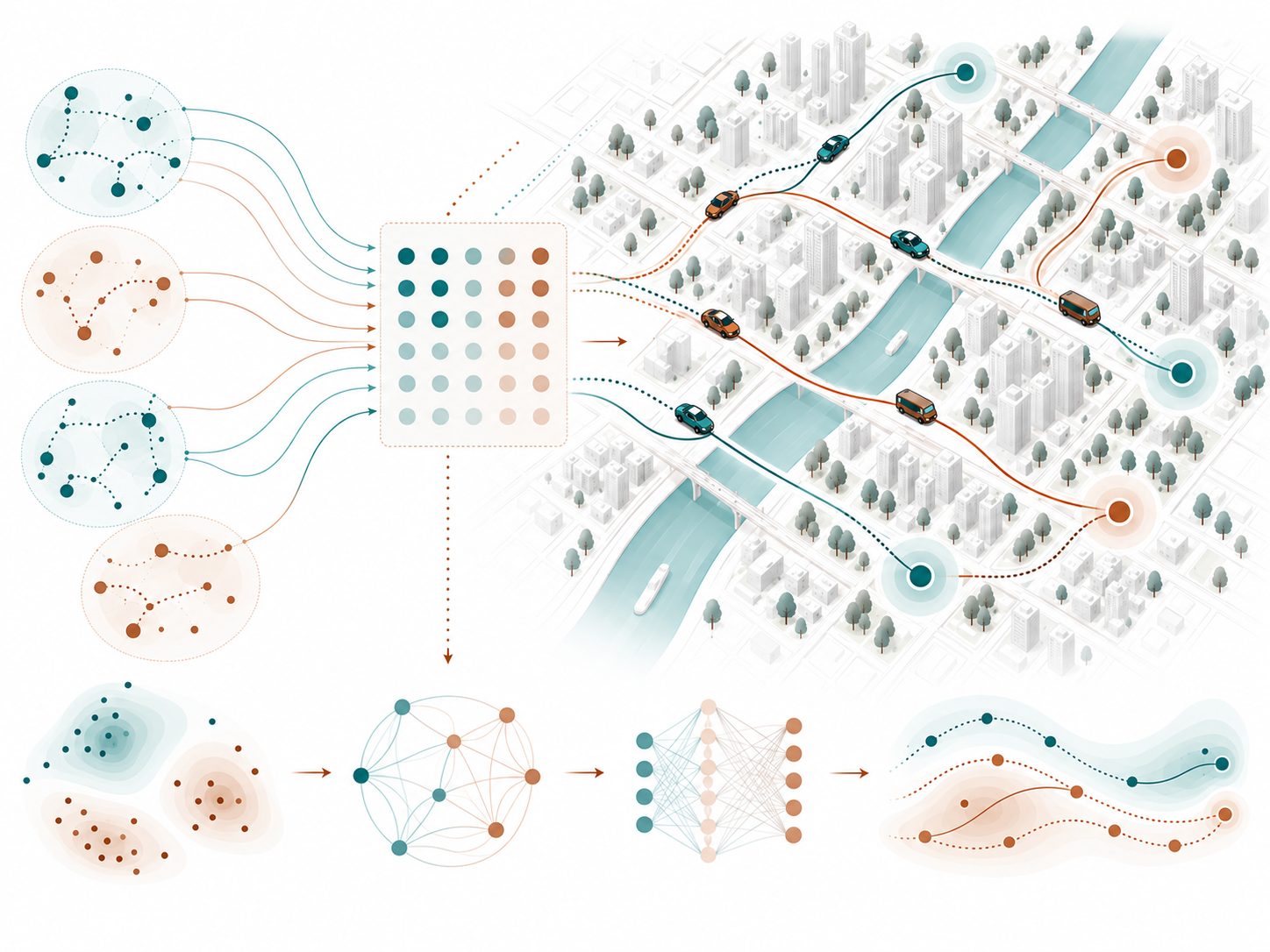
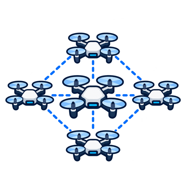
SALT turns a difficult fleet-level decision into two reusable pieces: learn how one agent can reach a target, then let optimal transport decide who should go where.

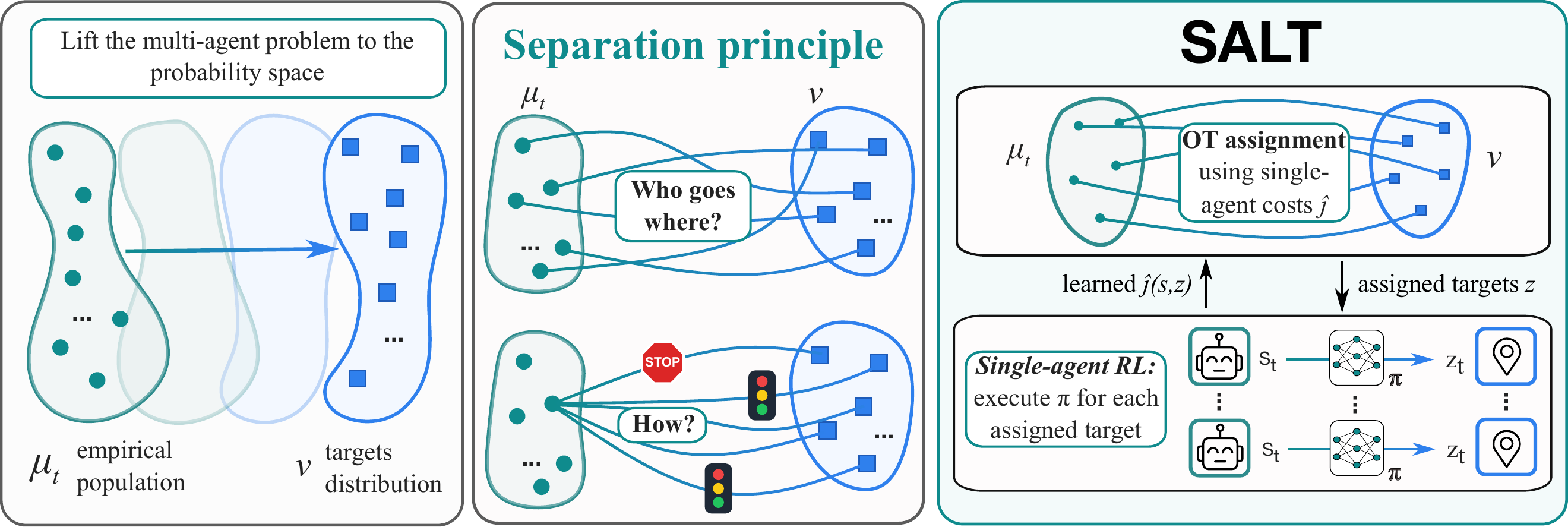
Three-stage SALT diagram showing the population-space formulation, separation principle, and optimal-transport assignment with single-agent reinforcement learning — From a population representation to the separation principle: optimal transport decides who goes where, while a shared single-agent policy decides how to reach each assigned target.

From one agent to a fleet

How SALT turns structure into an algorithm

01

Single-agent learning

Train a shared, target-conditioned policy and cost-to-go function for a single agent. Its complexity does not grow with the fleet size.

02

Optimal transport assignment

Use the learned target-conditioned cost-to-go function as the price of sending each agent to each target, and solve the resulting optimal-transport assignment.

03

Coordinate at scale

Route every agent with the same policy, while reusing the learned coordination layer for new target configurations and unseen fleet sizes.

Why separation is possible

The problem has just enough structure

Interchangeable agents

Agents are homogeneous: they share the same dynamics, costs, and policy. Their labels carry no useful information, so the problem can be lifted to the more natural space of probability measures.

Decoupled dynamics

Each agent moves under its own state, action, and noise. Agents are coupled through the collective goal, not through one another’s transition equations.

A distributional goal

The fleet aims to match a target distribution. Optimal transport measures the formation error and naturally exposes the assignment hidden inside the objective.

Possible applications

Where assignment and control meet

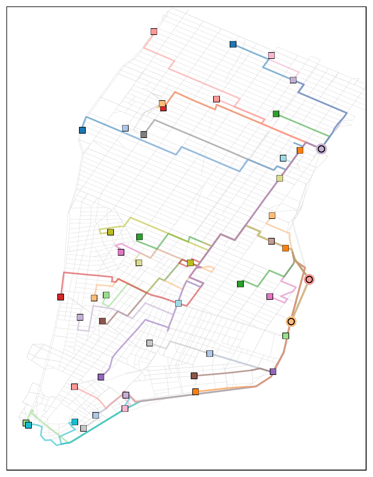
South Manhattan road network with colored vehicle routes connecting initial positions to delivery targets — Learned vehicle routes on the South Manhattan road network.

Main case study

Urban delivery fleets in South Manhattan

A dispatcher must decide both which vehicle should serve each request and how every vehicle should navigate through uncertain, time-varying traffic. SALT connects these decisions without learning a separate joint policy for every fleet size.

1

Assign using realistic costs

Optimal transport pairs vehicles and requests using the learned expected cost-to-go, not only geometric distance.

2

Route with one shared policy

Each vehicle follows the same target-conditioned policy toward its assigned destination.

3

Adapt as the city changes

Assignments can be recomputed online as traffic conditions, requests, or vehicle locations evolve.

2,087 intersections4,255 directed roads1-100 vehicles

More generally

Taxis navigating to passenger pickup locations

Ride-hailing

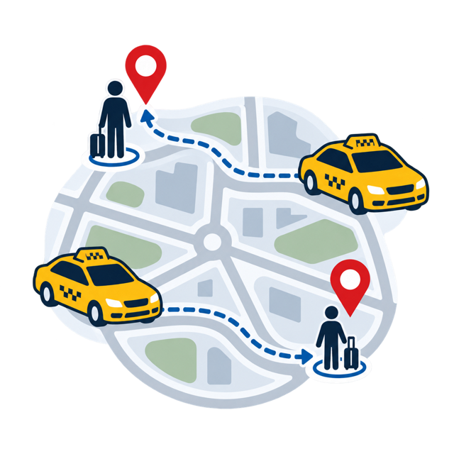
Match available drivers to changing passenger demand.

Autonomous warehouse robots carrying packages

Warehouse logistics

Assign mobile robots to shelves, parcels, and stations.

A coordinated formation of autonomous drones

Drone coverage

Coordinate inspection or sensing targets across a fleet.

Ambulance navigating toward an emergency location

Emergency response

Dispatch responders as incidents and priorities change.

Empirical results

One learner, fleets of different sizes

SALT coordinating vehicles on the time-varying South Manhattan road network.

Why this helps in practice: a conventional multi-agent policy learns in a joint state-action space whose size grows rapidly with the number of agents. SALT handles the only population-level decision through optimal transport, while trajectories from the entire fleet train one shared single-agent learner. We tested the algorithm on gridworld ablations and on a delivery task over south Manhathann

1–100fleet-size transfer in deployment without retraining

15–21%lower travel time than static shortest path on South Manhattan

480×fewer interactions than MAPPO to reach milestones in a gridworl environment

Model-Free Optimal Control

Data-Driven Linear Programs for Control

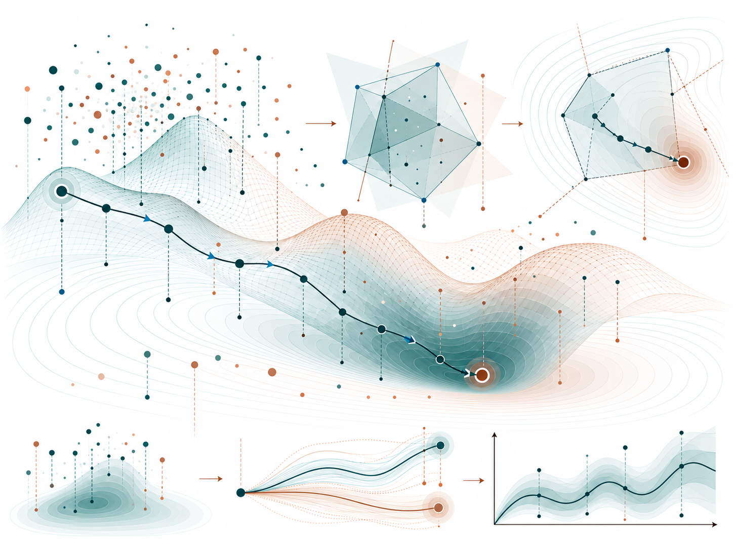
This work develops data-driven linear-programming methods for model-free optimal control in continuous state and action spaces. It characterizes when sampled optimal-control LPs remain bounded and uses moment-matching to design cost vectors that preserve finite solutions and useful control performance, including for nonlinear systems and limited datasets.

Optimal controlData-driven methodsLinear programming

Illustration of optimization landscapes, geometric structures, and probabilistic trajectories

The challenge in one sentence

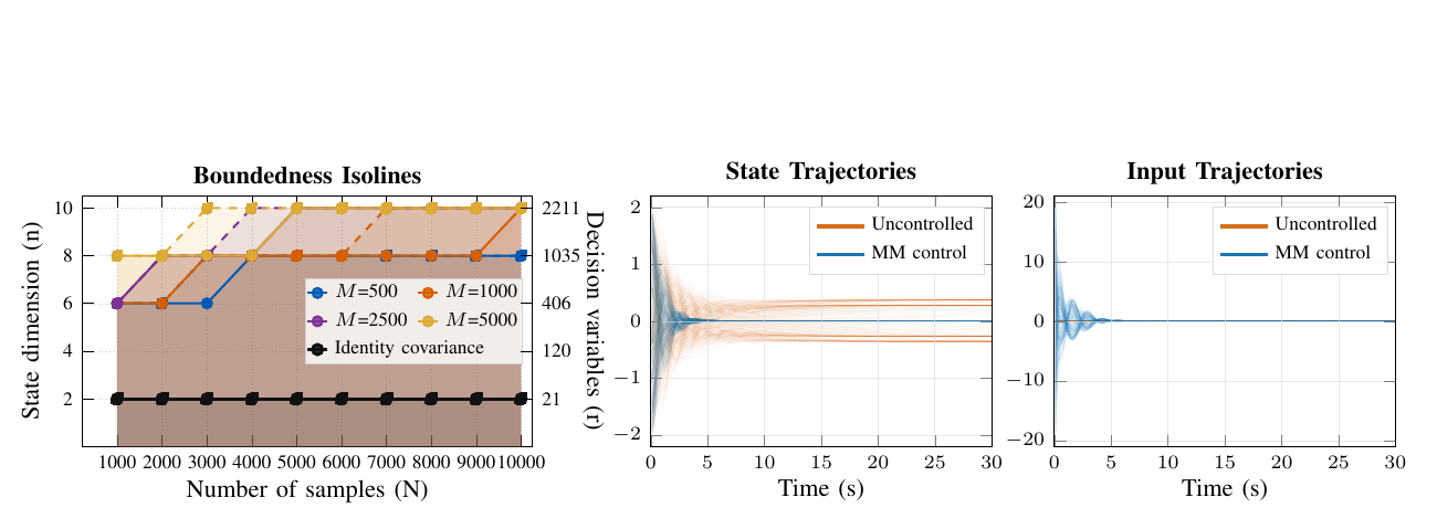
A sampled Bellman linear program may look perfectly feasible and still have no finite optimum. The missing ingredient is choosing an objective direction supported by the data.

observed data

(x_i,u_i,x_i^+,\ell_i)

sampled Bellman LP

\Phi^\top\alpha\leq\ell

finite optimum?objective geometry decides

From transitions to a controller

A four-step data-driven construction

01

Collect transitions

(x_i,u_i,x_i^+,\ell_i)

Observe state, action, next-state, and cost tuples without identifying the system dynamics.

02

Build the sampled LP

\Phi^\top \alpha \leq \ell

Use basis functions to turn sampled Bellman inequalities into a finite-dimensional linear program.

03

Match the moments

b_c = \Phi\lambda

Construct the objective from the same data geometry so that the optimization direction lies inside the bounded cone.

04

Extract a controller

\pi(x)=\arg\min_u q(x,u)

Solve the bounded LP and act greedily with respect to the learned Q-function.

Why the sampled LP can fail

Feasibility does not guarantee a finite solution

Finite data

Only finitely many Bellman inequalities are observed, leaving unconstrained directions in the approximate Q-function.

The objective matters

Unlike the exact LP, the sampled problem can be finite or unbounded depending on the selected cost vector.

Geometry decides boundedness

The observed transitions generate a cone of objective directions for which the LP has a finite optimum.

Boundedness characterization

\begin{aligned} b_c \in \operatorname{cone}(\Phi) &\iff \exists\,\lambda\geq 0 \\[-2pt] &\text{such that } b_c=\Phi\lambda \end{aligned}

The vector $b_c=\int \phi(z)c(dz)$ determines the direction in which the LP maximizes. Boundedness holds precisely when this vector can be represented as a nonnegative combination of the columns of the data matrix $\Phi$ . Moment matching constructs such a direction directly from the observed transitions.

No regularizer required: boundedness comes from objective design rather than clipping the feasible set.Polynomial features: the required moments can be obtained from a tractable linear or semidefinite feasibility problem.

Experimental evidence

Finite solutions that still control well

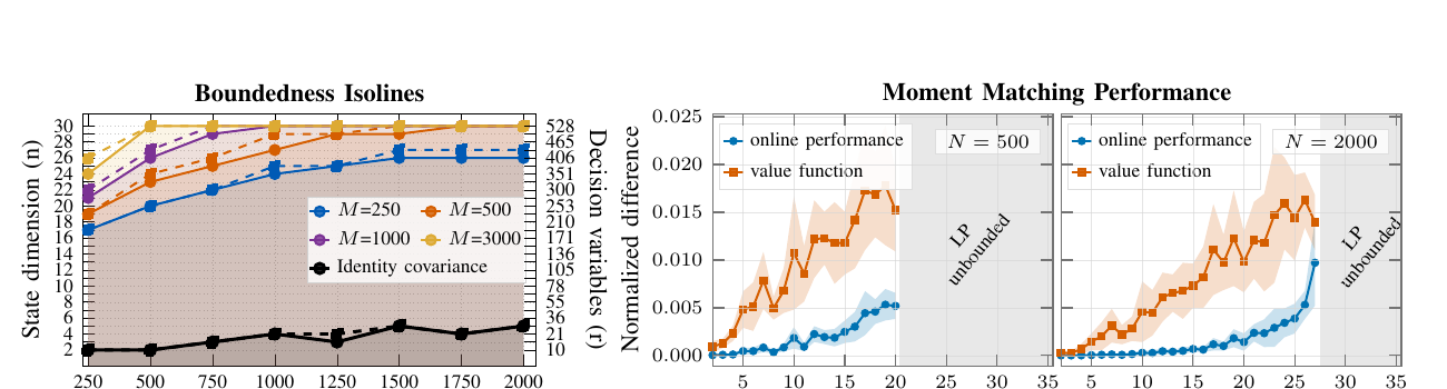
Boundedness isolines and normalized controller performance for linear systems — Moment matching remains bounded in substantially higher dimensions than a fixed-covariance objective while retaining near-optimal closed-loop performance.

Boundedness isolines and controlled state and input trajectories for nonlinear mechanical systems — The learned polynomial controller stabilizes the unstable equilibrium, whereas uncontrolled trajectories settle at other equilibria.

n = 30100% bounded at N = 500 in the tested LTI setting

≈1%closed-loop performance gap from analytic LQR

nonlinearpolynomial control from model-free transition data

Bayesian Machine Learning

Function-Space MCMC for Wide Neural Networks

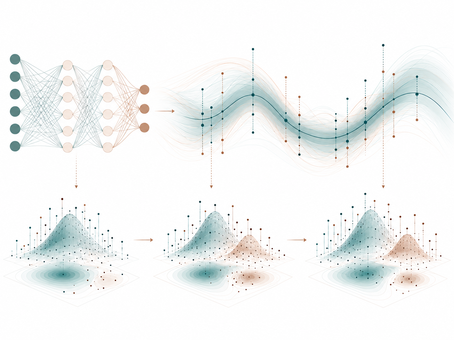
This work develops MCMC methods for Bayesian wide neural networks directly in function space. Using preconditioned Crank-Nicolson proposals and the Gaussian-process perspective of wide networks, it studies how to sample posterior functions and quantify uncertainty without making inference increasingly sensitive to parameter dimension.

Bayesian MLMCMCWide neural networks

Illustration of neural networks, trajectories, and probability landscapes for scalable multi-agent coordination